
We have already study a basic example of piecewise defined functions: step functions.

Now we are going to study piecewise functions where the pieces are not necessarily constant but linear. To start with we are going to consider only continuous piecewise linear functions. There is no discontinuity at each endpoint of the subdomains within that interval.
Continuous piecewise linear functions F and step functions f form pairs in some way.
A typical use of continuous piecewise linear functions is when we link several points in a graph using segments. This kind of approximation to a curve is known as Linear Interpolation.
Example of a continuous piecewise linear function is the definition of the absolute value function.
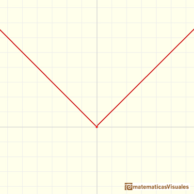
We can consider now the derivative of each piece (in this case, the derivative is the slope of the line) and we get a an step function.
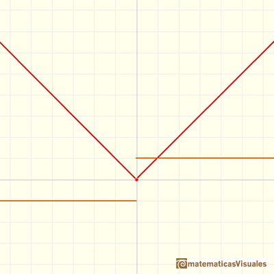
continuous piecewise linear functions are 'smooth almost everywhere'. There are only some points where the function is not smooth. They are examples of piecewise differentiable functions.
A function is piecewise differentiable if each piece is differentiable throughout its subdomain, even though the whole function may not be differentiable at the points between the pieces.
We remember that a linear function. The graph of a linear function is an straight line.
The derivative of a linear function is a basic example of derivative, it is a constant function.
The integral of a non-constant linear function is a quadratic function.

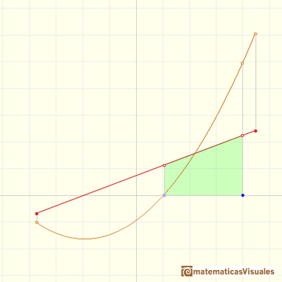
Now we are going to study the relation between a continuous piecewise linear function F and the step function f build with the slopes.
We can play with the applet and start with a function F:
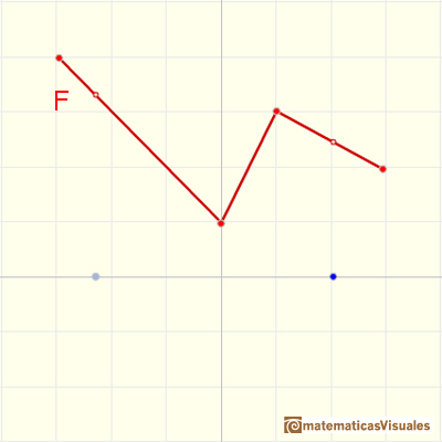
Then the slopes define an step function f (you can see this function as velocity):
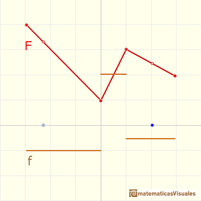
If you consider the area under this step function f ...
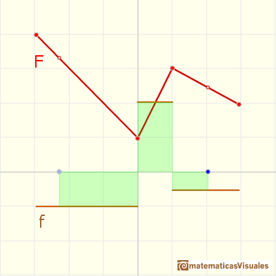
... you get a continuous linear piecewise function that is a vertical translation of the original piecewise function.
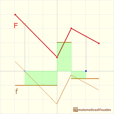
This process is called integration. The function you get is one integral function (you can see it as distance, if f is velocity).
Changing the origin of integration (blue point, to the right and left) you can translate the integral function up and down.
In the next applet, we start with an step function f and look for one continuous linear piecewise function F that have slopes equal to the initial step function. As you know, this process is integration.

You can drag up and down the blue dot to translate the integral function: there are infinite integral functions.
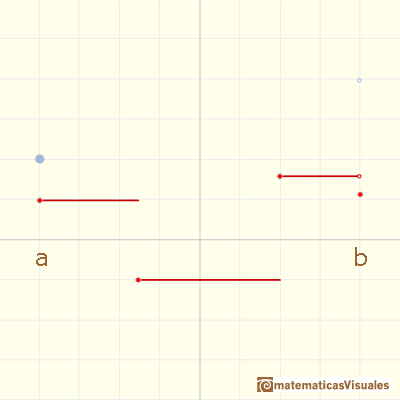
If F(a) is fixed you can consider the function F(x)
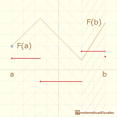
Suppose that you are asked about the value of F(b) and that the slopes of the different pieces are given.
Then you can calculate the values F(c), F(d) and F(b) using the point-slope formula for lines.
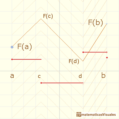
If there is a lot of pieces, you have to work hard to get F(b).
F(x) is an integral function. Then

This is the Fundamental Theorem of Calculus.
You can calculate the area piece by piece to get the integral
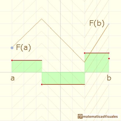
Or you can use the average value and remember that

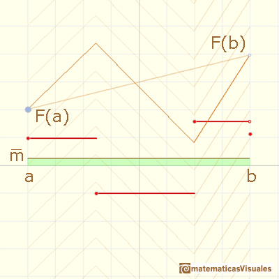
Now, this formula relates the Fundamental Theorem of Calculus with the point-slope formula:

We are going to integrate a continuous piecewise linear function.
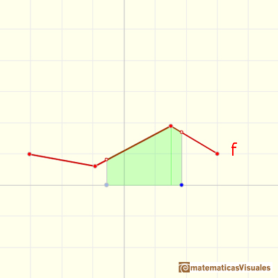
The integral function F(x) is made by several connected pieces of parabola.
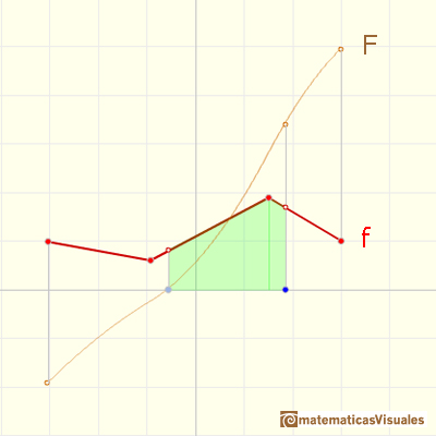
You can see that the connection of these pieces of parabola is smooth.
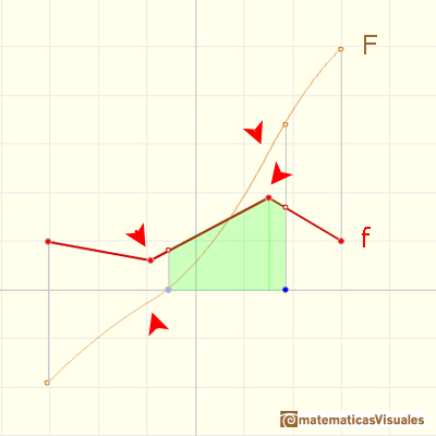
This function F(x) is not only continuous, it is differentiable. You can see that dragging the blue dot and moving the tangent. It changes smoothly. This is a general property: when f continuous then F is more than continuous, it is differentiable.
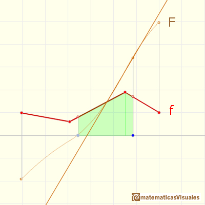
If we differentiate F we get the original function f again.

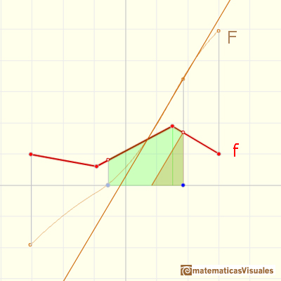
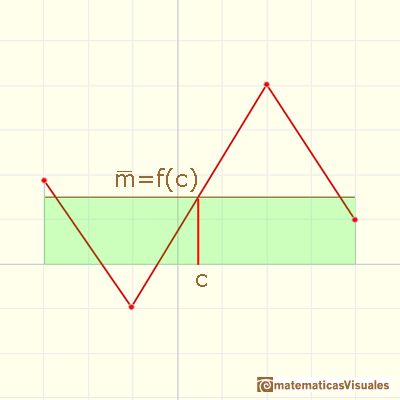
The average value of a function f(x) over the interval [a,b] is given by

In the next applet you can play with this concept.
As this functions are continuous, they are special cases of the Mean Value Theorem for integrals: If f(x) is a continuous function over the interval [a,b] then there is a number c in [a,b] such that

Next month we are going to study discontinuous piecewise linear functions.
REFERENCES
 NEXT
NEXT
 PREVIOUS
MORE LINKS


