Two points with different values of x determine a linear function (a polynomial of degree less or equal to 1)

The derivative of a lineal function is a constant function.
Three points not in a line determine a quadratic function, a parabola.
A quadratic function is a polynomial function of degree 2. They have the expression (standar form):
The graph of a quadratic function is a parabola.
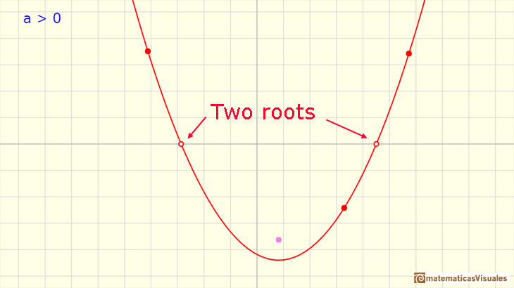
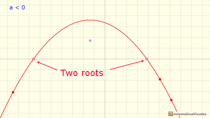
Some parabolas cut the x-axis in two points. We call this points the roots (or zeros) of the polynomial.
We can obtain these roots solving the quadratic equation
The solutions of a quadratic equation are given by:
The discriminant is defined as:
If the discriminant is greater than 0 the quadratic equation has two roots, x1, x2. Then we can
write a quadratic function in the factored form:
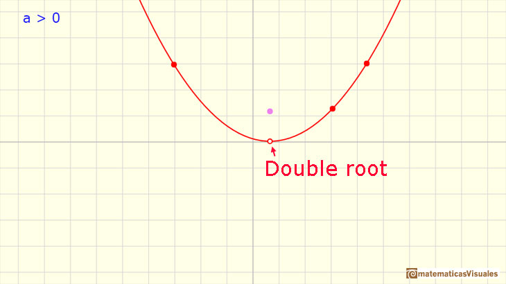
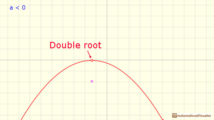
Some parabolas only cut (or touch) the x-axis in one point.
In this case the discriminant is equal to zero and the
solution of the quadratic equation is:
Then we say that this root is a double root. In this case, the quadratic function in the factored form is:
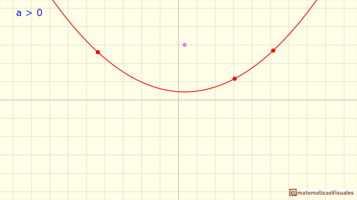
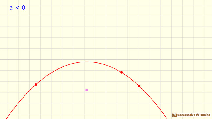
Some parabolas do not cut the x-axis. In this case, the discriminant is less than 0 and the quadratic equation has no
real solution.
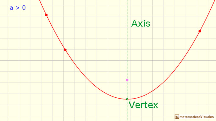
When a is a positive number the parabola opens upward but if a is a negative number the parabola opens downward. Here
we can see one example with two real roots, one with only one root and one with no real roots:
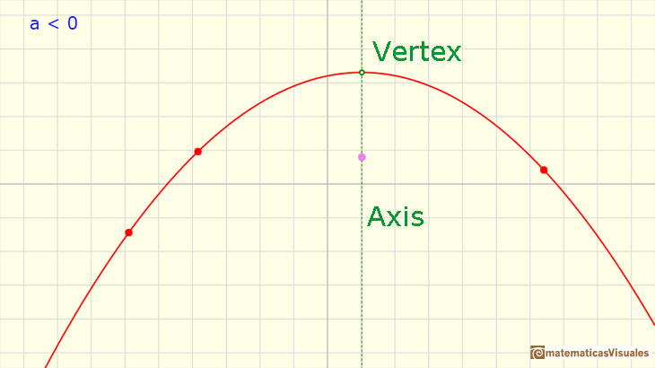
Every parabola has a maximum or a minimum (it is a maximum if a is a negative number and it is a minimum if a is a positive number). This point is called the vertex. The vertical line through the vertex is the
axis of symmetry of the parabola. The equation of the axis is:
The vertex of the parabola is the point with coordinates:
Parabolas are conic sections:
Quadratic Functions with real or complex coefficients always have two roots (real or complex) (Fundamental Theorem of Algebra):
REFERENCES
Michael Spivak, 'Calculus', Third Edition, Publish-or-Perish, Inc.
Tom M. Apostol, 'Calculus', Second Edition, John Willey and Sons, Inc.
I.M. Gelfand, E.G. Glagoleva, E.E. Shnol, 'Functions and Graphs', Dover Publications, Mineola, N.Y.
MORE LINKS

Power with natural exponents are simple and important functions. Their inverse functions are power with rational exponents (a radical or a nth root)

We can consider the polynomial function that passes through a series of points of the plane. This is an interpolation problem that is solved here using the Lagrange interpolating polynomial.
The derivative of a lineal function is a constant function.

The derivative of a quadratic function is a linear function, it is to say, a straight line.

As an introduction to Piecewise Linear Functions we study linear functions restricted to an open interval: their graphs are like segments.

A piecewise function is a function that is defined by several subfunctions. If each piece is a constant function then the piecewise function is called Piecewise constant function or Step function.

A continuous piecewise linear function is defined by several segments or rays connected, without jumps between them.

The derivative of a cubic function is a quadratic function, a parabola.

Rational functions can be writen as the quotient of two polynomials. Linear rational functions are the simplest of this kind of functions.

When the denominator of a rational function has degree 2 the function can have two, one or none real singularities.

Lagrange polynomials are polynomials that pases through n given points. We use Lagrange polynomials to explore a general polynomial function and its derivative.

If the derivative of F(x) is f(x), then we say that an indefinite integral of f(x) with respect to x is F(x). We also say that F is an antiderivative or a primitive function of f.

The integral concept is associate to the concept of area. We began considering the area limited by the graph of a function and the x-axis between two vertical lines.

Monotonic functions in a closed interval are integrable. In these cases we can bound the error we make when approximating the integral using rectangles.

If we consider the lower limit of integration a as fixed and if we can calculate the integral for different values of the upper limit of integration b then we can define a new function: an indefinite integral of f.

It is easy to calculate the area under a straight line. This is the first example of integration that allows us to understand the idea and to introduce several basic concepts: integral as area, limits of integration, positive and negative areas.

To calculate the area under a parabola is more difficult than to calculate the area under a linear function. We show how to approximate this area using rectangles and that the integral function of a polynomial of degree 2 is a polynomial of degree 3.

We can see some basic concepts about integration applied to a general polynomial function. Integral functions of polynomial functions are polynomial functions with one degree more than the original function.

The Fundamental Theorem of Calculus tell us that every continuous function has an antiderivative and shows how to construct one using the integral.

The Second Fundamental Theorem of Calculus is a powerful tool for evaluating definite integral (if we know an antiderivative of the function).

By increasing the degree, Taylor polynomial approximates the exponential function more and more.

By increasing the degree, Taylor polynomial approximates the sine function more and more.

The function is not defined for values less than -1. Taylor polynomials about the origin approximates the function between -1 and 1.

The function has a singularity at -1. Taylor polynomials about the origin approximates the function between -1 and 1.

The function has a singularity at -1. Taylor polynomials about the origin approximates the function between -1 and 1.

This function has two real singularities at -1 and 1. Taylor polynomials approximate the function in an interval centered at the center of the series. Its radius is the distance to the nearest singularity.

This is a continuos function and has no real singularities. However, the Taylor series approximates the function only in an interval. To understand this behavior we should consider a complex function.

Complex power functions with natural exponent have a zero (or root) of multiplicity n in the origin.

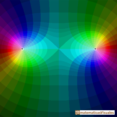
A polynomial of degree 2 has two zeros or roots. In this representation you can see Cassini ovals and a lemniscate.

A complex polinomial of degree 3 has three roots or zeros.

Every complex polynomial of degree n has n zeros or roots.


 NEXT
NEXT

 PREVIOUS
