
The Normal distribution is a very important example of a continuous random variable (the variable can take any real value).
We can use the Normal distribution as a tool for computing probabilities. For example, a normal curve can be used as an approximation of binomial probabilities.

The probability density function of a normal distribution is shaped like a bell and it is symmetrical about its mean. The total area under the normal curve is 1.
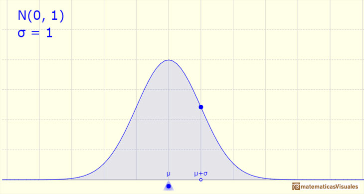
The density is concentrated around the mean and becomes very small by moving from the center to the left or to the right of the distribution (the so called "tails" of the distribution). The further a value is from the center of the distribution, the less probable it is to observe that value.
Two parameters determine a normal distribution: the mean and the standard deviation.
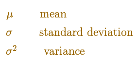
If a probability variable follows a normal distribution we can write:

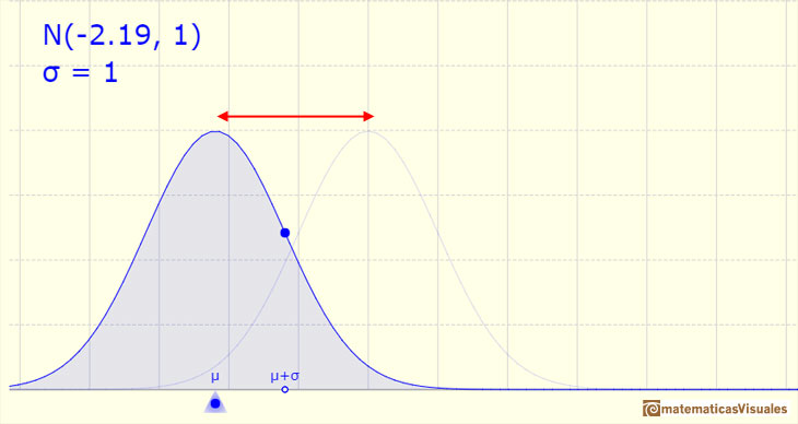
The mean of the distribution determines the location of the center of the graph.
By changing the mean the shape of the graph does not change, but the graph is translated to the right or to the left.
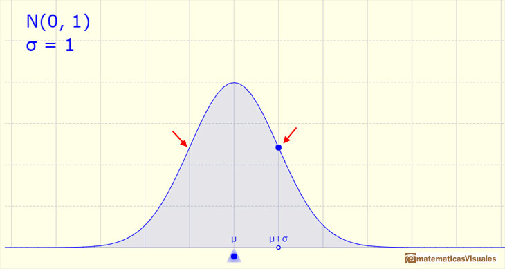
The density function has two inflection points, located one standard deviation away from the mean.
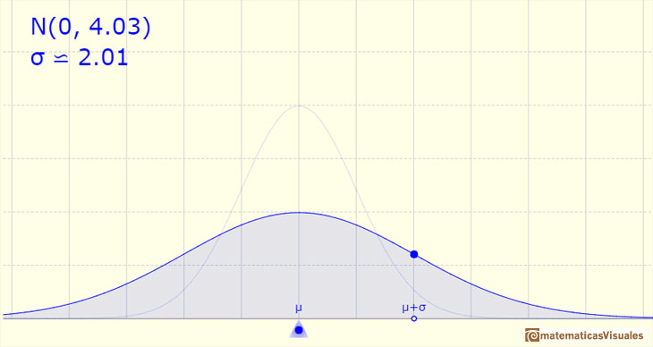
By increasing the standard deviation, (if the mean is the same, then the center of the graph does not change), the shape of the graph changes, the curve es wide, the dispersion is high (The higher the standard deviation the greater the variable dispersion).
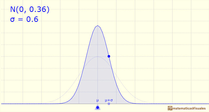
If the standard deviation is small, the curve is tall and narrow.
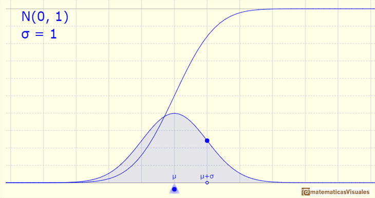
The simplest example is called the Standard Normal Distribution. It is a special case, when the mean is equal to 0 and the variance is 1.

The (cumulative) distribution function has an S-shape.
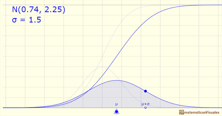
The standard normal distribution function gives the probability that a standard normal variable assumes a value less than x.

We can modifying the parameters of the normal distribution.
The mean is represented by a triangle that can be seen as an equilibrium point. By dragging it we can modify the mean.
Dragging the point on the curve (which is one of the two inflexion points of the curve) we modify the standard deviation.
We can see the cumulative distribution function and how it change by modifiyng the mean (simple translation) and the standard deviation (reflecting greater or lesser dispersion of the variable).
The red dots control the vertical and horizontal scales of the graphic.
The Normal distribution was studied by Gauss (1809). Gauss derived the normal distribution mathematically as the probability distribution of the error of measurements, which he called the normal law of errors. Before Gauss: de Moivre(1738) and Laplace (1774).
REFERENCES
 NEXT
NEXT
 PREVIOUS
MORE LINKS


